Objective:
Southern Utah County has multiple small towns that are experiencing significant growth; two of these, Woodland Hills and Elk Ridge, don't currently have easy access to highways that connect to other areas of Utah County. As the populations of these cities continue to expand, it will become more difficult for existing roadways to accommodate increased traffic flow, and it will be frustrating for drivers who have to take roundabout routes to get to larger urban areas. In order to remedy this, I was asked to find an optimal route for an expressway that would connect I-15 and Highway 6. This website is to detail the methods and data I used, and to show the resulting proposed route.
factors:
There were a few things that played into defining the best route for the expressway, known as the "least-cost path." Least-cost here refers to the path that will have the lowest cost based on environmental, monetary, and temporal factors:
- the slope of the terrain
- the value of each parcel of land
- where wetlands are located
- what preexisting roads can be used
I also had five "destinations," areas that I hoped to connect with the expressway, and a "source" area that the expressway would travel through.
DATA:
I obtained the data for each of these factors online. It included maps showing roads, the boundary of each parcel of land, etc., as shown below. The data also included information about things such as the owner, market value, and size of the parcels and how large the roads were.
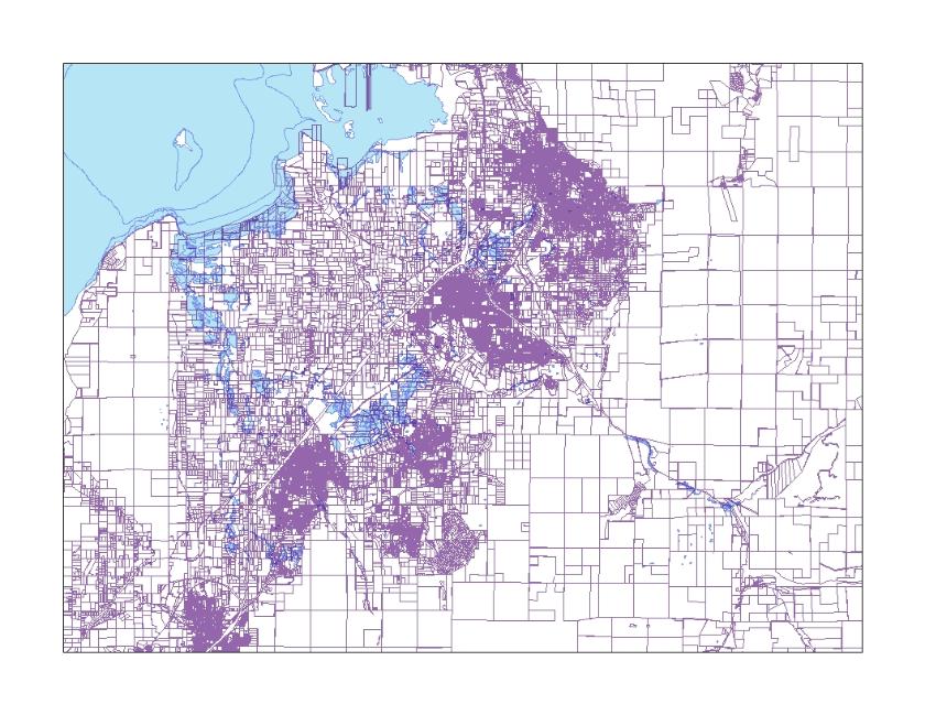
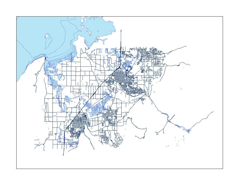
These maps show examples of the raw data obtained online. The map to the right shows the outline of tax parcels; notice that they are significantly smaller and more dense in some areas - these are urban areas. The map to the left shows the roads that go through the area I'm focusing on. Both include Utah Lake in the upper left corner as well as the outline of wetlands that go through the study area.
Map showing tax parcels and wetlands layers
Map showing roads and wetlands layers
methods:
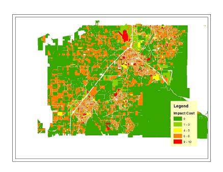
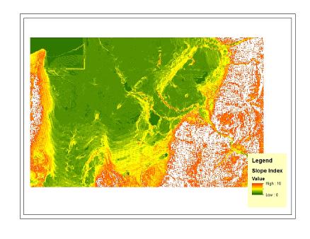
Once I had the data, I began to analyze them. This analysis process involved a few steps. I took each factor, such as the parcel value, and "scored" them. In the case of the parcels, this meant giving each parcel a score of 1-10, with 1 being the cheapest parcels of land and 10 being the most expensive. This is shown in the map below on the left. The map on the right shows the cost score of the slope. The steeper slopes are shown in orange with a higher cost than flatter areas shown in green. The white indicates mountainous ranges too steep to even be considered for the road.
A similar analysis was performed on the roads and wetlands as well; larger roads were given a lower cost score since the expressway could connect with these preexisting roads to lower cost, while rural roads that would require substantial construction in order to be used were given a higher cost. The wetlands were a little different because they don't have concrete boundaries; thus, areas closer to the wetland were given a higher score, while scores gradually decreased further away from the wetland areas.
Map showing the impact cost of tax parcels
Map showing the impact cost of slope
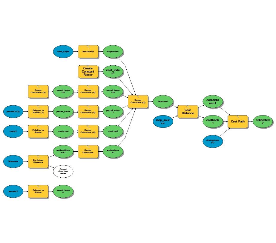
After all the data was given a score, I needed to combine all of these factors -the parcels, the wetlands, the roads, and the slope- into one overall value for the land. A model, shown below, was used to do this.
In this model, the blue circles are raw data. The yellow squares show the tools that I used to run my analysis, and the green circles are the output of those analyses. To get the value of all of the scores put together, I calculated their average. This is the part of the model where six green circles -the factors- come together into one yellow square, called "Raster Calculator 2." This calculator is where their average was figured. Then I "calibrated" my model. This calibration was a process of figuring out if there were some factors -slope, for example- that should be weighted more heavily than others to get a feasible path.
Model used to run analyses
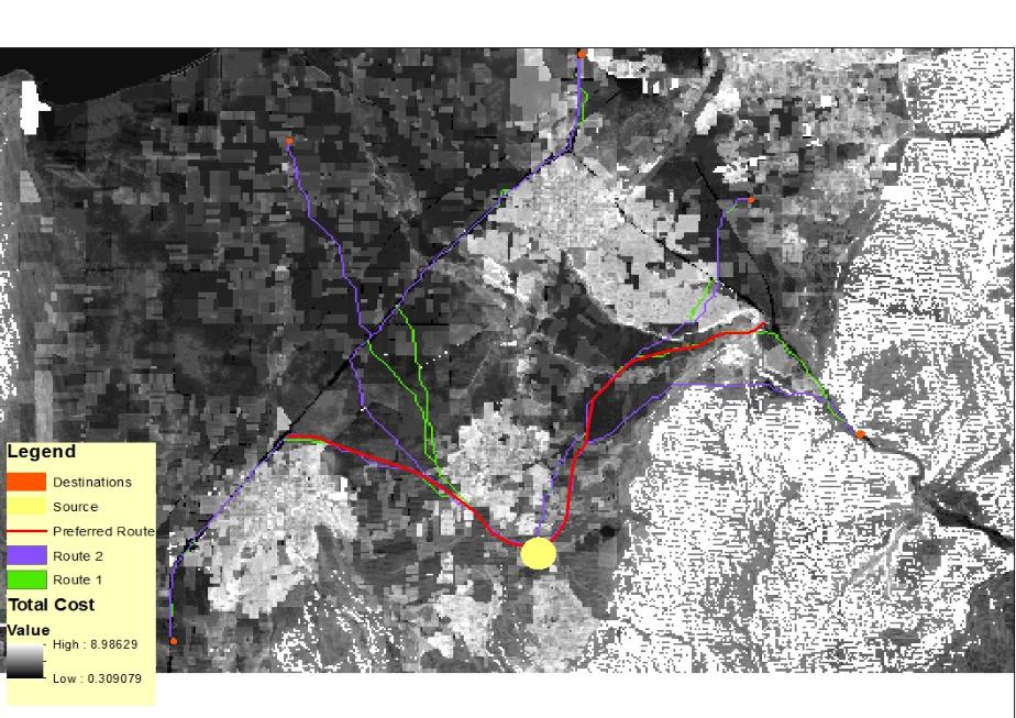
After this calibration was complete and all of the factors had been accounted for, I got a map that showed the overall cost for the land as well as the computer's calculated lowest cost routes to the five destinations from the source area. This is shown in the map below. The darker areas indicate the higher cost urban areas, and the white once again represents the areas of the mountains where a road would simply not be feasible.
Map showing total land cost, computer model routes, and hand-drawn route with destinations and source
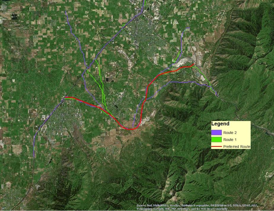
Finally, after the model had calculated the least-cost path, it was still up to me to decide which one of those paths was the best and to make any changes I thought necessary -for instance, if I thought the computer's route was on an area that was too steep to be practical. I also had to make sure that the curves of the road would not be dangerous on a fast-moving road, and that the expressway would fit into existing highways. Below, the green and purple routes are the ones created by the computer, and the red is the route that I designed.
Map showing computer model routes and hand-drawn final route
conclusions:
In the interactive map below, I've explained where I would put intersections and overpasses, and which existing roads I would demolish. I've also showed how the on and off ramps would work. I tried to gauge how much traffic would use each intersection and based my choice on whether to make that an intersection or overpass on that estimate. There were two sections where I differed significantly from the computer's paths. One was to avoid a steep area in the east side of the study area, and the other was to go through a golf course rather than a neighborhood towards the eastern end of the highway. Both locations are marked by yellow crosses on the interactive map below.
Interactive web-map